Statistical intervals are staples of the quality and validation practitioner’s statistical tool box. Statistical intervals can manifest as plus-or-minus limits on test data, represent a margin of error in a scientific poll, or indicate the level of confidence associated with a predicted value. But what exactly do all these intervals mean? Why do we need them? This is the first part of a three-part series written to help validation and quality practitioners understand the three most common intervals; namely, the confidence interval, the prediction interval, and the tolerance interval. In this part, confidence intervals are discussed.
Confidence intervals are the best known and most often used of the statistical intervals. Confidence intervals are used to express the uncertainty associated with a population parameter such as the population mean, µ, or the population standard deviation, s. In the pharmaceutical industry, confidence intervals are often used to express the uncertainty of an analytical result.
Usually when a number of samples are collected to represent a population, the data are averaged to yield an estimate of the true population mean. However, because the number of observations used to calculate the sample average is usually much smaller than the population itself; the sample average can only be considered an estimate of the true population mean. The true population mean may be equivalent to the sample mean, but may also be located about the sample mean as shown in Figure 1.
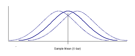
locations of the population distribution.
The uncertainty of knowing the location of the true population mean can be expressed numerically by calculating a confidence interval about the sample mean. A two-sided confidence interval is depicted graphically in figure 2.
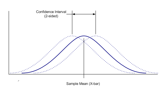
Confidence intervals for population means are relatively straight forward to calculate. A two-sided confidence interval for a population mean is defined as:
x̄±t1-a/2:n-1where x̄ is the sample average, s the sample standard deviation, n is the sample size, 1-a is the desired confidence level, and t1-a/2:n-1 is the 100(1-a/2) percentile of the t distribution with n-1 degrees of freedom.
The Student’s t distribution is a continuous probability distribution similar to the normal distribution. The Student’s t distribution is typically used in place of the normal distribution when the sample sizes are small. Tables listing critical values for the Student's t distribution can be found in most statistics textbooks
Most tables of critical values for the Student’s t distribution are arranged in cross-tabulated fashion where the table rows correspond to the number of degrees of freedom, n, and the table columns correspond to the desired 1-a confidence level. To find the critical value, one merely has to locate the critical value corresponding to the intersection of the number of degrees of freedom and the desired confidence level. For single parameter estimates, the degrees of freedom is equal to one less the sample size or n-1.
Suppose for example, that an analyst is tasked with measuring the pH of ten samples taken from a batch of liquid product. The measurements yield the following pH data:
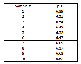
The average pH, x̄, in this example is 6.52; the sample standard deviation, s, is 0.11. The analyst wants to report the estimated mean pH along with a statement of the uncertainty of this estimate. Using a = 0.05 (confidence level = 95%), the analyst calculates a two-sided limit. For a two-sided limit, the critical value for the t distribution is found using one-half of the value for a; that is, 0.05/2 = 0.025. This value along with the degrees of freedom (n-1= 9 in this case) will be used to look up the critical value of the t distribution. The critical value in this example is 2.262. Entering this value into the two sided confidence interval formula gives:

The lower interval bound in this example is 6.52 - 0.08 = 6.44; the upper bound is 6.52 + 0.08 = 6.60. The interval range is 0.16.
Typically, confidence intervals are calculated using a probability of 100(1-a) = 95%; however, any probability value may be used. Using a larger probability value will yield a wider interval as well as greater confidence in the parameter estimate; conversely, a smaller probability value will yield a narrower interval, but provide less confidence in the estimate. Sample size also affects the width of the confidence interval due to the increasing effect of the √nand n-1 terms in the confidence interval formula. For a given confidence level, using a larger sample size will yield a smaller interval width.
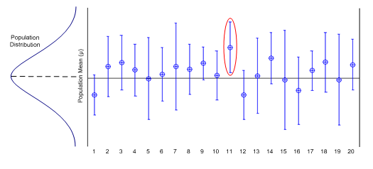
Just as important as knowing how to calculate a confidence interval is correctly interpreting the interval once it has been calculated. Confidence intervals are commonly interpreted to mean that there is an x% probability that the true population mean is located within the interval. This interpretation however, is not quite correct. The correct interpretation is that in independent sample sets, 100(1-a)% of the calculated intervals will cover the true parameter value.
Figure 3 demonstrates this interpretation graphically. Figure 3 is an interval plot of 20 simulated sample sets of known mean and standard deviation. The plot was generated with a = 0.05. As can be seen in the plot, the known mean falls within 19 of the 20 intervals. The single interval in which the mean does not fall corresponds to 5% of the intervals not expected to cover the true population mean.
Sometimes there is only an upper or a lower specification limit associated with the parameter of interest. Perhaps an analyst wants to know with a given confidence that the mean purity of a substance is greater than a specified lower limit. Because there is no upper limit on how pure the substance can be, we can calculate a single-sided confidence interval that will provide a lower bound on the region likely to contain the true parameter value. To calculate single-sided confidence intervals one simply substitutes a for a/2 in the two-sided confidence interval formula defined above. The upper and lower confidence interval bounds are defined then as,
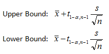
One-sided confidence intervals bracket the true parameter value on only one side and should only be used when one is interested in quantifying the uncertainty of a parameter estimate with respect to a one-sided specification. For two-sided specifications, the two-sided confidence interval formula should be used.
Because confidence intervals express the uncertainty associated with a population parameter and not the population as a whole, confidence intervals yield the narrowest uncertainty region compared to the other interval types. As such, confidence intervals should only be used when the closeness of the population mean or variance to a prescribed target value is the primary goal.
In addition to knowing the uncertainty associated with a population parameter, there are also situations where we are interested in knowing beforehand where a next observation is likely to fall. Intervals indicating such a region are known as prediction intervals. This type of interval will be discussed in Part II of the article.
- Fred Wiles, Project Lead, ProPharma
July 10th, 2013
Interested in learning more? Contact us today to find out how we can help with your global regulatory needs.
References
- NIST/SEMATECH e-Handbook of Statistical Methods, Pyzdek, Thomas. (2000). The Six Sigma Handbook. New York, New York: McGraw-Hill Companies, Inc.
TAGS: Statistical Intervals Process Validation Life Science Consulting
